ISMIP-HOM

Benchmark Experiments for Higher-Order Ice Models

Conveners Which models can participate? What type of experiments? Documents Input data files: Haut Glacier d'Arolla Presentations Results of the benchmark The ISMIP webpage The EISMINT webpage

FULL TEXT (PDF) Description of the experiments

Conveners

Frank PATTYN, Laboratoire de Glaciologie, Départment des Sciences de la Terre et de l'Environnement, Université Libre de Bruxelles, CP 160/03, Av. F.D. Roosevelt 50, 1050 - Bruxelles (email: fpattyn@ulb.ac.be)

Tony PAYNE, Bristol Glaciology Centre, School of Geographical Sciences, University of Bristol, Bristol B88 1SS, England (email: a.j.payne@bristol.ac.uk)

Which models can participate?

The tests proposed below were defined and partly discussed during the International Symposium on Physical and Mechanical Processes in Ice in relation to Glacier and Ice-sheet Modelling, held in Chamonix Mont-Blanc, France, 26-30 August 2002 and during a first coordination meeting, held in Brussels, Belgium, June 3 and 4, 2003. The purpose of these tests is to fix benchmarks for future modelling attempts and to detect eventual weaknesses in numerical approaches of higher-order models. The experiments may be somewhat restrictive and may not be appropriate for all kinds of models.

During former model intercomparison exercises (EISMINT 1 and 2), a number of benchmarks were proposed for ice sheet models as well as for ice shelf models. The bulk of these ice-sheet models were based on the so-called shallow-ice approximation (SIA). In this exercise we will focus on so-called higher-order models, i.e. models that incorporate further mechanical effects, principally longitudinal stress gradients, or the full Stokes system. With longitudinal stresses we basically mean all stress components apart from the two horizontal plane shear components (Hindmarsh, 2004).

We tried to make the experiments accessible for many types of models, i.e. flowline models, vertically integrated planform models, as well as full three-dimensional models. The experiments are valid for both finite difference (FD) and finite element (FE) models. Furthermore, the grid type (regular or not) is unimportant.

All thermomechanical effects are neglected and an isotherm ice mass is considered. Experiments include ideal geometry tests as well as a real case experiment on Haut Glacier d'Arolla. The experiments are designed for the following types of higher-order models:

• 3D models: HHVF and HHVC, i.e. 2 horizontal dimensions and one vertical dimension. F = FULL (first, second-order, or solution of the full Stokes equations); C = CHANNEL (only solution for horizontal velocity v_x in the direction of the ice flow x). For C-type models, the stress field should include both vertical shear t_xz as well as longitudinal stresses t_xx and their gradients. F-type models also include t_yz, t_yy and t_xy (higher-order models). All stress gradients are included in the full Stokes models.

• 2D planform models: HHF, i.e. 2 horizontal dimensions but integrated over the vertical, in the sense that they. These models are basically ice-shelf models, but should be extended with a friction coefficient so that ice-stream flow can be simulated as well (so-called shelfy-stream model, e.g. MacAyeal, 1993).

• 2D flowline models: HVF and HVC, i.e. one horizontal dimension (in the direction of the ice flow) and one vertical dimension. The stress field should include both vertical shear t_xz as well as longitudinal stresses t_xx. The models considered are flowline models (HVF) which eventually include a parameterization of the width of the flowline, or channel models (HVC).

What type of experiments?

With exception of experiment F, all experiments are diagnostic, i.e. time evolution is not considered. This means that for a given geometry of the ice mass, a Glen-type flow law, and given appropriate boundary conditions, the stress and velocity field can be calculated. Experiment F considers time-dependent response (the experiment is run until the free surface and velocity field reach a steady state) for a constant viscosity (linear flow law). For this experiment analytical solutions exists that are developed by Gudmundsson (2003).

For experiments A-D, the model domain is square. The minimum number of grid points is not predefined. It is advised that people use a discretization scheme for which they think that the best possible results are obtained. Since this might be model dependent, we allow everyone to choose the number of grid points in the horizontal as well as in the vertical direction. The basic parameter for the experiments is the length scale of the domain L. Experiments are carried out for L = 160, 80, 40, 20, 10 and 5 km, respectively. These theoretical experiments are designed in such a way that variations in bed topography or friction coefficient are periodic, so that periodic boundary conditions to the velocity field apply.

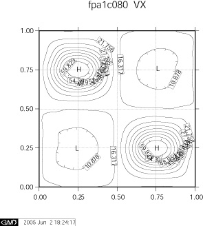
All experiments described below were tested with a HHVF and a HVF model (Pattyn, 2002; 2003). The examples shown here are based on a grid of 41 by 41 grid points in both horizontal directions x and x, and 41 vertical layers in z. Horizontal gridsize for the shown experiment L = 80 is Dx = 2051.282051 m. These results should be regarded as illustrations, as the discretization scheme is not considered to be optimal.

Experiment A: : ice flow over a bumpy bed

Model types: HHVF and HHVC

The bedrock topography consists of a series of sinusoidal bumps with an amplitude of 500 m. Both ice thickness and bedrock topography form an inclined plane in the x direction, so that the mean ice thickness of the model domain is 1600 m. Examples of the resulting surface velocity field are also shown below.

Experiment B: ice flow over a rippled bed

Model types: HHVF, HHVC, HVF and HVC

The only difference with experiment A is that the basal topography does not vary with y, so that the experiment is suitable for 2D flowline models as well. The basal topography is thus formed by a series of ripples with an amplitude of 500 m.

Experiment C: Ice stream flow I

Model types: HHVF, HHVC and HHF

The experiment is similar to experiment A, albeit that the bedrock topography is defined as an inclined plane parallel to the surface, so that ice thickness remains constant for the whole domain. The friction coefficient is prescribed as a sinusoidal function. Examples of the resulting surface velocity field are also shown below.

Experiment D: Ice stream flow II

Model types: HHVF, HHVC, HHF, HVF and HVC

The only difference with experiment C is that the basal friction coefficient does not vary with y, so that the experiment is suitable for 2D flowline models as well. The basal friction field is thus formed by a series of ripples. Below is a figure of the friction coefficient for this experiment.

Experiment E

Model types: HVF and HVC

Experiment E is a diagnostic experiment along the central flowline of a temperate glacier in the European Alps (Haut Glacier d'Arolla). Input for the model is formed by the longitudinal surface and bedrock profiles of Haut Glacier d'Arolla, Switzerland. The longitudinal profile of this glacier has a very simple geometry, hence the resulting stress field is not influenced by geometrical perturbations such as the presence of a steep ice fall. A zero basal velocity is considered, and the width of the drainage basin, is kept equal to 1 along the whole flowline domain, so that HVC and HVF models should give similar results. The flow-law rate factor A is taken constant over the whole model domain. Two experiments will be carried out, one without basal sliding and one with a small zone of zero traction. The input data file is found below.

Experiment F

Model types: HHVF and HHVC

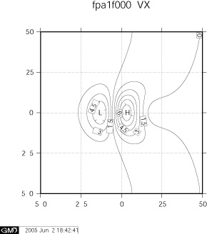
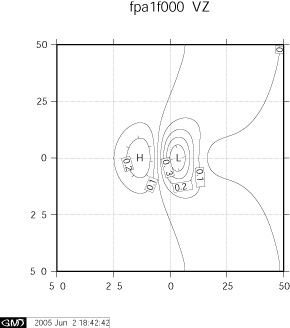
Experiment F is a prognistic experiment for which the free surface is allowed to relax until a steady state is reached for a zero surface mass balance. A complete description of this experiemnt is given in the PDF document. Below are examples of the relaxed surface elevation and velocity at the surface for the ice flow over a Gaussian perturbation (bump) with a slip ratio of zero (ice frozen to the bedrock).

Documents

PDF with full description of the experiments

Input data file: Haut Glacier d'Arolla

The basic input dataset of the Haut Glacier d'Arolla longitudinal profile is a flowline of 5 km in length with a grid spacing of 100 m, based on the topography of 1930. The file is an ASCII tabulated file containing 4 columns: (1) distance from the head (in meter), (2) bedrock topography (m a.s.l.), (3) the glacier surface (m a.s.l.), and (4) the zone of zero traction in the second experiment (marked by 1, otherwise 0). This zone starts at x = 2200m and ends at x = 2500m. Boundary conditions for all long profiles are zero ice thickness at either end. The file can be uploaded below.

Presentations

The official launch of the ISMIP-HOM experiments took place at the EGU Meeting in Vienna (2-7 April 2006). A poster was presented in the session CR13: Modelling ice sheets and glaciers: Pattyn, F and Payne, A.J. Ice Sheet Model Intercomparison Project: Benchmark Experiments for Higher-Order Ice Sheet Models (ISMIP-HOM) (CR13-1FR2P-0302). The abstract can be downloaded from:

http://www.cosis.net/abstracts/EGU06/04969/EGU06-J-04969.pdf

Preliminary results of the experiments were presented at a splinter meeting at EGU the year after in April 2007. A powerpoint presentation shows the results from all participants. The same results were also presented at the EGU meeting in a poster. The poster corresponds to the following abstract:

http://www.cosis.net/abstracts/EGU2007/01351/EGU2007-J-01351-1.pdf

Results

Results of the benchmark experiment were published in The Cryosphere:

http://www.the-cryosphere.net/2/95/2008/tc-2-95-2008.html

The numerical results of the participants can be downloaded from here (zipped files) as well as from The Cryosphere website: tc-2-95-2008-supplement.

The paper can be downloaded from: http://www.the-cryosphere.net/2/95/2008/tc-2-95-2008.pdf or from the link HERE.